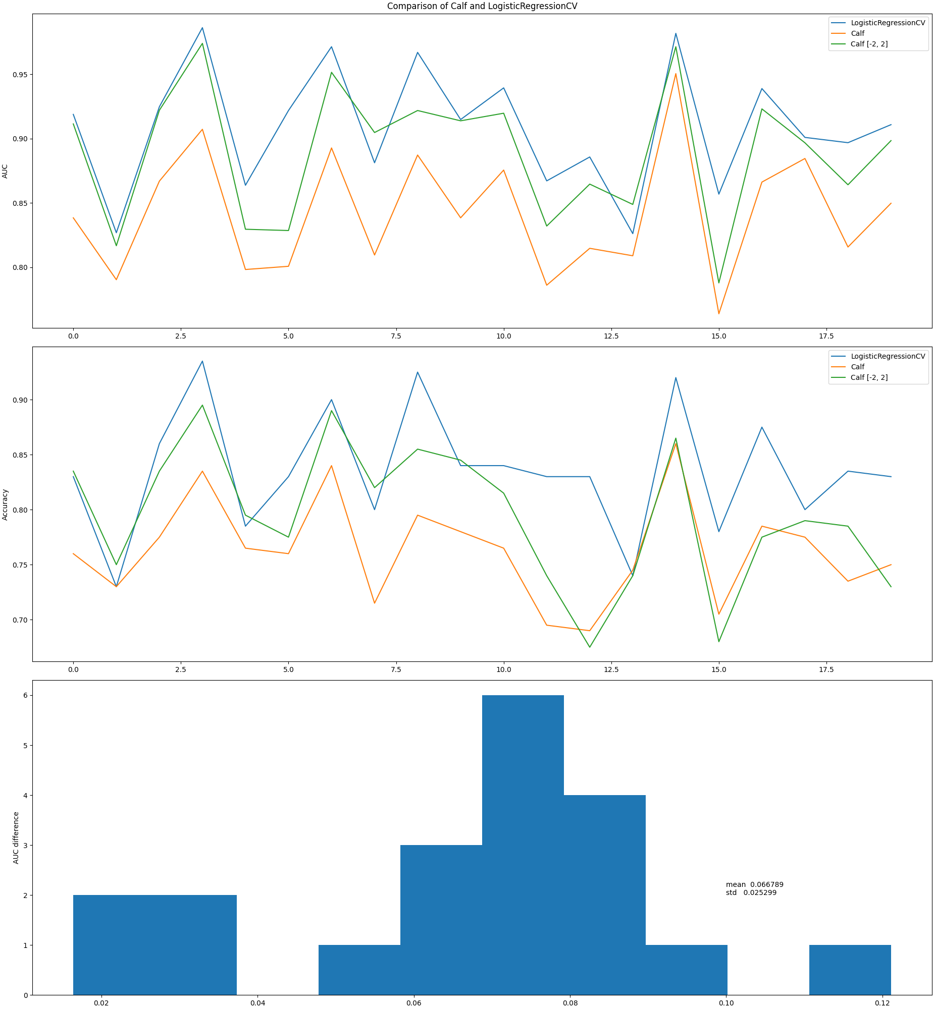
Compare Calf with LogisticRegression

A comparison of LogisticRegressionCV and Calf over 20 synthetic classification problems. Using the grid [-2, 2] with increments of .1, Calf improves upon Calf over the default grid, and in some cases, surpasses LogisticRegressionCV. The histogram at the bottom of the plot shows mean and standard deviation of the difference between LogisticRegressionCV and Calf.

import numpy as np
import pandas as pd
from matplotlib import pyplot as plt
from sklearn.datasets import make_classification
from sklearn.linear_model import LogisticRegressionCV
from sklearn.metrics import accuracy_score, roc_auc_score
from sklearn.preprocessing import StandardScaler

from calfcv import Calf


methods = [
    ('Logit', LogisticRegressionCV(max_iter=10000)),
    ('Calf', Calf()),
    ('Calf [-2, 2]', Calf(grid=np.arange(-2, 2, .1))),
]

score = {}
for desc, _ in methods:
    score[desc] = {}
    score[desc]['AUC'] = []
    score[desc]['Accuracy'] = []

rng = np.random.RandomState(11)
for _ in range(20):
    # Make a classification problem
    X, y_d = make_classification(
        n_samples=200,
        n_features=40,
        n_informative=10,
        n_redundant=5,
        n_classes=2,
        hypercube=True,
        random_state=rng
    )
    scaler = StandardScaler()
    X_d = scaler.fit_transform(X)

    for desc, clf in methods:
        lp = clf.fit(X_d, y_d).predict_proba(X_d)
        auc = roc_auc_score(y_true=y_d, y_score=clf.fit(X_d, y_d).predict_proba(X_d)[:, 1])
        acc = accuracy_score(y_true=y_d, y_pred=clf.fit(X_d, y_d).predict(X_d))
        score[desc]['AUC'].append(auc)
        score[desc]['Accuracy'].append(acc)

# compare the mean of the differences of auc
diff = np.subtract(score['Logit']['AUC'], score['Calf']['AUC'])
df_describe = pd.DataFrame(diff)

# plot the results
fig, axs = plt.subplots(3, 1, layout='constrained')
xdata = np.arange(len(score['Logit']['AUC']))
axs[0].plot(xdata, score['Logit']['AUC'], label='LogisticRegressionCV')
axs[0].plot(xdata, score['Calf']['AUC'], label='Calf')
axs[0].plot(xdata, score['Calf [-2, 2]']['AUC'], label='Calf [-2, 2]')

axs[0].set_title('Comparison of Calf and LogisticRegressionCV')
axs[0].set_ylabel('AUC')
axs[0].legend()

axs[1].plot(xdata, score['Logit']['Accuracy'], label='LogisticRegressionCV')
axs[1].plot(xdata, score['Calf']['Accuracy'], label='Calf')
axs[1].plot(xdata, score['Calf [-2, 2]']['Accuracy'], label='Calf [-2, 2]')
axs[1].set_ylabel('Accuracy')
axs[1].legend()

axs[2].hist(diff)
axs[2].set_ylabel('AUC difference')
stats = pd.DataFrame(diff).describe().loc[['mean', 'std']].to_string(header=False)
axs[2].text(.1, 2, stats)
fig.set_size_inches(18.5, 20)
plt.show()