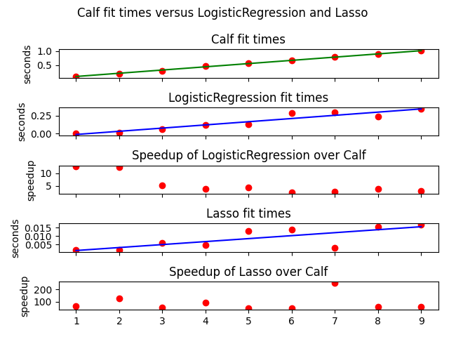
Calf runtime complexity

A classifier runtime comparison plot including Calf. Lasso is much faster than LogisticRegression, which in turn is faster than Calf. The calculation of AUC dominates the Calf runtime.

import time

import matplotlib.pyplot as plt
import numpy as np
from sklearn.datasets import make_classification
from sklearn.linear_model import Lasso, LogisticRegression

from calfcv import Calf

ts = {'calf': [], 'lr': [], 'las': []}
ns = np.arange(1, 10, 1)
for i in ns:
    X, y = make_classification(
        n_samples=100 * i,
        n_features=20 * i,
        n_informative=10 * i,
        n_redundant=5 * i,
        n_classes=2,
        random_state=11
    )

    ts['calf'].append(Calf().fit(X, y).fit_time_)

    start = time.time()
    cls1 = LogisticRegression(max_iter=10000).fit(X, y)
    elapsed = time.time() - start
    ts['lr'].append(elapsed)

    start = time.time()
    cls2 = Lasso(max_iter=10000).fit(X, y)
    elapsed = time.time() - start
    ts['las'].append(elapsed)

degree = 1

# stack vertically, share the same x-axis
# figure = plt.figure(figsize=(10, 10))
fig, ax = plt.subplots(5, sharex=True)
fig.suptitle('Calf fit times versus LogisticRegression and Lasso ')

coeffs = np.polyfit(ns, ts['calf'], degree)
p = np.poly1d(coeffs)
ax[0].plot(ns, ts['calf'], 'or')
ax[0].plot(ns, [p(n) for n in ns], '-g')
ax[0].set_ylabel('seconds')
ax[0].set_title('Calf fit times')

coeffs = np.polyfit(ns, ts['lr'], degree)
p = np.poly1d(coeffs)
ax[1].plot(ns, ts['lr'], 'or')
ax[1].plot(ns, [p(n) for n in ns], '-b')
ax[1].set_ylabel('seconds')
ax[1].set_title('LogisticRegression fit times')

ax[2].plot(ns, np.divide(ts['calf'], ts['lr']), 'or')
ax[2].set_title('Speedup of LogisticRegression over Calf')
ax[2].set_ylabel('speedup')

coeffs = np.polyfit(ns, ts['las'], degree)
p = np.poly1d(coeffs)
ax[3].plot(ns, ts['las'], 'or')
ax[3].plot(ns, [p(n) for n in ns], '-b')
ax[3].set_ylabel('seconds')
ax[3].set_title('Lasso fit times')

ax[4].plot(ns, np.divide(ts['calf'], ts['las']), 'or')
ax[4].set_title('Speedup of Lasso over Calf')
ax[4].set_ylabel('speedup')

plt.tight_layout()
plt.show()