Analysis of data that lacks informative features
Build a pipeline to analyze the N2 dataset. These results are an example of what you can find when the data lacks informative features.
[108]:
import numpy as np
import pandas as pd
from sklearn.preprocessing import StandardScaler
from sklearn.pipeline import Pipeline
from sklearn.model_selection import train_test_split, GridSearchCV
import matplotlib.pyplot as plt
import math
from sklearn.linear_model import RidgeCV
import warnings
[109]:
# Ignore warnings
warnings.filterwarnings('ignore')
[110]:
input_file_path = "../../../data/n2.csv"
df = pd.read_csv(input_file_path, header=0, sep=",")
[111]:
X = df.loc[:, df.columns != 'ctrl/case']
[112]:
y = df['ctrl/case'].astype('int').tolist()
features = df.columns
[113]:
print(y)
[0, 0, 0, 0, 0, 0, 0, 0, 0, 0, 0, 0, 0, 0, 0, 0, 0, 0, 0, 0, 0, 0, 0, 0, 0, 0, 0, 0, 0, 0, 0, 0, 0, 0, 0, 0, 0, 0, 0, 0, 1, 1, 1, 1, 1, 1, 1, 1, 1, 1, 1, 1, 1, 1, 1, 1, 1, 1, 1, 1, 1, 1, 1, 1, 1, 1, 1, 1, 1, 1, 1, 1]
Feature importance from coefficients
None of the features are important
[114]:
ridge = RidgeCV(alphas=np.logspace(-6, 6, num=5)).fit(X, y)
importance = np.abs(ridge.coef_)

# Find the 5 most important coefficients and features
# Operate on the coefficients and features as tuples
# maintain the association as they are sorted and selected.
tup = list(zip(importance, features))
tup = sorted(tup,  key=lambda x: abs(x[0]), reverse=True)
tup = [x for x in tup[:5] if not math.isclose(x[0], 0)]
importance, features = list(zip(*tup))

plt.bar(height=importance, x=features)
plt.title("Feature importances via coefficients")
plt.show()
Try to learn from all the features
[115]:
# the number of permutations during a permutation test
num_permutations = 1000
[116]:
from sklearn.linear_model import Lasso

pipeline = Pipeline([
    ('scaler', StandardScaler()),
    ('model', Lasso())
])
[117]:
parametersGrid = {
    "model__alpha": np.arange(0.01, 2, .1)
}

search = GridSearchCV(
    pipeline,
    parametersGrid,
    scoring="roc_auc",
    cv=5,
    verbose=False
)
Train the classifier
[118]:
search.fit(X, y)
[118]:
GridSearchCV(cv=5,
             estimator=Pipeline(steps=[('scaler', StandardScaler()),
                                       ('model', Lasso())]),
             param_grid={'model__alpha': array([0.01, 0.11, 0.21, 0.31, 0.41, 0.51, 0.61, 0.71, 0.81, 0.91, 1.01,
       1.11, 1.21, 1.31, 1.41, 1.51, 1.61, 1.71, 1.81, 1.91])},
             scoring='roc_auc', verbose=False)
In a Jupyter environment, please rerun this cell to show the HTML representation or trust the notebook. On GitHub, the HTML representation is unable to render, please try loading this page with nbviewer.org.
GridSearchCV(cv=5,
             estimator=Pipeline(steps=[('scaler', StandardScaler()),
                                       ('model', Lasso())]),
             param_grid={'model__alpha': array([0.01, 0.11, 0.21, 0.31, 0.41, 0.51, 0.61, 0.71, 0.81, 0.91, 1.01,
       1.11, 1.21, 1.31, 1.41, 1.51, 1.61, 1.71, 1.81, 1.91])},
scoring='roc_auc', verbose=False)Pipeline(steps=[('scaler', StandardScaler()), ('model', Lasso())])StandardScaler()
Lasso()
[119]:
search.best_params_
[119]:
{'model__alpha': 0.01}
[120]:
search.score(X, y)
[120]:
1.0
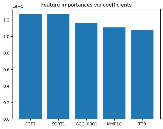
Coefficients and features from the best fit
[121]:
import math
import pprint

coefficients = search.best_estimator_.named_steps['model'].coef_
tup = list(zip(coefficients, features))
tup = sorted(tup,  key=lambda x: abs(x[0]), reverse=True)
tup = [x for x in tup if not math.isclose(x[0], 0)]
pprint.pprint(tup)
[(-0.09687810936109993, 'TTR'),
 (0.0887806299222524, 'MMP10'),
 (0.07456955839378693, 'SORT1'),
 (-0.04847222854397004, 'FGF2')]
Permutation Tests
[122]:
# Add random features and the classifier score should go down.
n_uncorrelated_features = 20
rng = np.random.RandomState(seed=0)
# Use same number of samples as in the psych data and 20 features
X_rand = rng.normal(size=(X.shape[0], n_uncorrelated_features))
Permutation test over the data, and data including random features
[123]:
from sklearn.model_selection import StratifiedKFold
from sklearn.model_selection import permutation_test_score

clf = search
cv = StratifiedKFold(2, shuffle=True, random_state=0)

score_psych, perm_scores_psych, pvalue_psych = permutation_test_score(
    clf, X, y, cv=cv, n_permutations=num_permutations, scoring="roc_auc", verbose=False
)

score_rand, perm_scores_rand, pvalue_rand = permutation_test_score(
    clf, X_rand, y, cv=cv, n_permutations=num_permutations, scoring="roc_auc", verbose=False)
[124]:
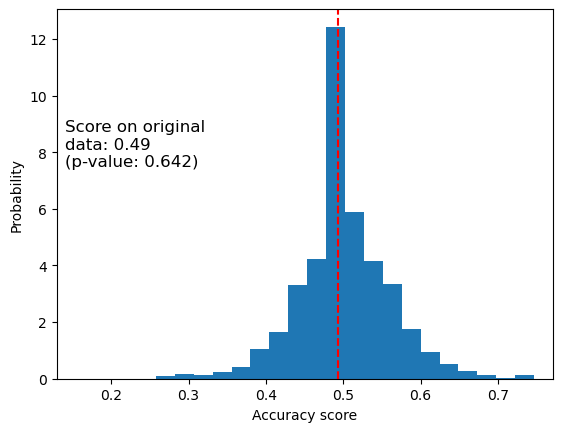
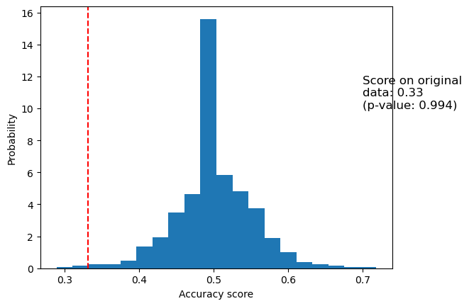
import matplotlib.pyplot as plt

fig, ax = plt.subplots()

ax.hist(perm_scores_psych, bins=20, density=True)
ax.axvline(score_psych, ls="--", color="r")
score_label = f"Score on original\ndata: {score_psych:.2f}\n(p-value: {pvalue_psych:.3f})"
ax.text(0.7, 10, score_label, fontsize=12)
ax.set_xlabel("Accuracy score")
_ = ax.set_ylabel("Probability")
[125]:
_, ax = plt.subplots()

ax.hist(perm_scores_rand, bins=20, density=True)
ax.set_xlim(0.13)
ax.axvline(score_rand, ls="--", color="r")
score_label = f"Score on original\ndata: {score_rand:.2f}\n(p-value: {pvalue_rand:.3f})"
ax.text(0.14, 7.5, score_label, fontsize=12)
ax.set_xlabel("Accuracy score")
ax.set_ylabel("Probability")
plt.show()
Try to learn from the features selected by an F-test
[126]:
from sklearn.feature_selection import SelectFromModel
from sklearn.svm import LinearSVC
from sklearn.linear_model import LogisticRegression
from sklearn.linear_model import Lasso
from sklearn.feature_selection import SelectKBest, f_classif

sfm_lsvc = SelectFromModel(LinearSVC(penalty="l1", dual=False, max_iter=10000))
sfm_lr = SelectFromModel(LogisticRegression(dual=False, solver='liblinear', max_iter=10000))

skb = SelectKBest(f_classif, k=5)

pipeline = Pipeline([
    ('scaler', StandardScaler()),
    ('feature_selection', skb),
    ('model', Lasso())
])
[127]:
# Look at the parameters revealed by get_params and see which items to include in the grid
parametersGrid = {
    "model__alpha": np.arange(0.01, 2, .1)
}

search = GridSearchCV(
    pipeline,
    parametersGrid,
    scoring="roc_auc",
    cv=5,
    verbose=False
)
Train the classifier
[128]:
search.fit(X, y)
[128]:
GridSearchCV(cv=5,
             estimator=Pipeline(steps=[('scaler', StandardScaler()),
                                       ('feature_selection', SelectKBest(k=5)),
                                       ('model', Lasso())]),
             param_grid={'model__alpha': array([0.01, 0.11, 0.21, 0.31, 0.41, 0.51, 0.61, 0.71, 0.81, 0.91, 1.01,
       1.11, 1.21, 1.31, 1.41, 1.51, 1.61, 1.71, 1.81, 1.91])},
             scoring='roc_auc', verbose=False)
In a Jupyter environment, please rerun this cell to show the HTML representation or trust the notebook. On GitHub, the HTML representation is unable to render, please try loading this page with nbviewer.org.
GridSearchCV(cv=5,
             estimator=Pipeline(steps=[('scaler', StandardScaler()),
                                       ('feature_selection', SelectKBest(k=5)),
                                       ('model', Lasso())]),
             param_grid={'model__alpha': array([0.01, 0.11, 0.21, 0.31, 0.41, 0.51, 0.61, 0.71, 0.81, 0.91, 1.01,
       1.11, 1.21, 1.31, 1.41, 1.51, 1.61, 1.71, 1.81, 1.91])},
scoring='roc_auc', verbose=False)Pipeline(steps=[('scaler', StandardScaler()),
('feature_selection', SelectKBest(k=5)), ('model', Lasso())])StandardScaler()
SelectKBest(k=5)
Lasso()
[129]:
search.best_params_
[129]:
{'model__alpha': 0.01}
[130]:
search.score(X, y)
[130]:
0.8031250000000001
Coefficients and features from the best fit
[131]:
import math
import pprint

coefficients = search.best_estimator_.named_steps['model'].coef_
tup = list(zip(coefficients, features))
tup = sorted(tup,  key=lambda x: abs(x[0]), reverse=True)
tup = [x for x in tup if not math.isclose(x[0], 0)]
pprint.pprint(tup)
[(0.15477039712201454, 'SORT1'),
 (0.13381633055236333, 'TTR'),
 (0.1025959132389977, 'FGF2'),
 (0.037155677196843345, 'MMP10'),
 (0.029658349600763394, 'GCG_0001')]
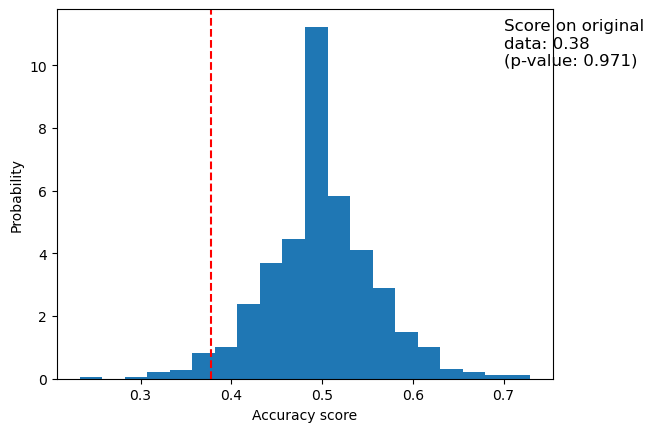
Features selected by the F-test
[132]:
idx = search.best_estimator_.named_steps['feature_selection'].get_support(indices=True)
best_feature_names = [df.columns[i] for i in idx]
best_feature_names
[132]:
['FAS', 'MMP10', 'CCL2', 'SORT1', 'FGF2']
Permutation Tests
[133]:
# Add random features and the classifier score should go down.
n_uncorrelated_features = 20
rng = np.random.RandomState(seed=0)
# Use same number of samples as in the psych data and 20 features
X_rand = rng.normal(size=(X.shape[0], n_uncorrelated_features))
Permutation test over the data, and data including random features
[134]:
from sklearn.model_selection import StratifiedKFold
from sklearn.model_selection import permutation_test_score

clf = search
cv = StratifiedKFold(2, shuffle=True, random_state=0)

score_psych, perm_scores_psych, pvalue_psych = permutation_test_score(
    clf, X, y, cv=cv, n_permutations=num_permutations, scoring="roc_auc", verbose=False
)

score_rand, perm_scores_rand, pvalue_rand = permutation_test_score(
    clf, X_rand, y, cv=cv, n_permutations=num_permutations, scoring="roc_auc", verbose=False)
[135]:
import matplotlib.pyplot as plt

fig, ax = plt.subplots()

ax.hist(perm_scores_psych, bins=20, density=True)
ax.axvline(score_psych, ls="--", color="r")
score_label = f"Score on original\ndata: {score_psych:.2f}\n(p-value: {pvalue_psych:.3f})"
ax.text(0.7, 10, score_label, fontsize=12)
ax.set_xlabel("Accuracy score")
_ = ax.set_ylabel("Probability")
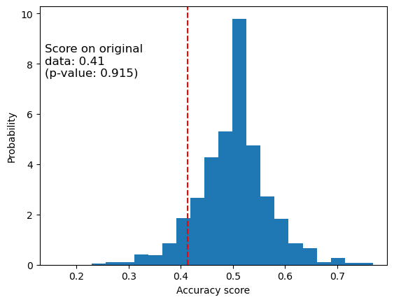
[136]:
_, ax = plt.subplots()

ax.hist(perm_scores_rand, bins=20, density=True)
ax.set_xlim(0.13)
ax.axvline(score_rand, ls="--", color="r")
score_label = f"Score on original\ndata: {score_rand:.2f}\n(p-value: {pvalue_rand:.3f})"
ax.text(0.14, 7.5, score_label, fontsize=12)
ax.set_xlabel("Accuracy score")
ax.set_ylabel("Probability")
plt.show()