The N2 dataset

The N2 dataset provides features that are hypothesized to be informative for a progression to psychosis. This notebook provides an overview of N2.

# Author: Rolf Carlson, Carlson Research LLC, <hrolfrc@gmail.com>
# License: 3-clause BSD

import pandas
from sklearn.linear_model import LogisticRegression
from sklearn.metrics import RocCurveDisplay
from sklearn.metrics import roc_auc_score
import matplotlib.pyplot as plt
import math
from sklearn.model_selection import train_test_split

Get the input file path from the calf project

input_file_path = "../../../data/n2.csv"

Read the input file into a DataFrame

df = pandas.read_csv(input_file_path, header=0, sep=",")
df.head()

	ctrl/case	ADIPOQ	SERPINA3	AMBP	A2M	ACE	AGT	APOA1	APOA2	APOA4	...	CALCA	IL6	LTA	CSF3	PGF	GCG_0001	IL1B	TGFB3	FGF2	MDA-LDL
0	0	1.1538	-1.008	0.4650	-0.6181	-0.9350	1.7169	0.974	1.7821	-0.2580	...	-0.3688	0.8739	-0.2390	2.8335	0.4469	0.101	0.1688	-0.1861	1.9591	-0.0720
1	0	-0.7661	-1.039	1.2479	0.2220	-0.7140	2.6709	-0.275	0.1680	0.9759	...	-0.3688	1.5408	3.5482	-0.6669	-0.7770	1.015	0.1688	0.2689	-0.3498	-0.5491
2	0	-0.2721	-0.766	-0.7480	-1.0371	0.0459	-0.2940	0.046	0.9320	-0.5050	...	0.2562	0.2060	-0.8099	-0.6669	-0.7770	0.372	-0.5152	-0.1861	-0.3498	-0.5491
3	0	-0.8201	-1.281	0.4650	-0.1980	0.8059	0.8980	-0.954	-0.4270	-0.5050	...	-0.3688	-0.5718	-0.8099	-0.6669	-0.5050	-0.543	0.1688	0.2689	-0.5978	-0.5491
4	0	0.0019	-1.188	-0.7090	0.6421	0.2039	-0.3500	-0.275	0.5070	0.2349	...	0.0612	1.8737	1.0388	-0.6669	0.4469	0.575	-0.2332	-0.4131	0.4472	-0.5491

5 rows × 136 columns

Remove the outcome column to get the independent variables

X = df.loc[:, df.columns != 'ctrl/case']
X.head()

	ADIPOQ	SERPINA3	AMBP	A2M	ACE	AGT	APOA1	APOA2	APOA4	APOH	...	CALCA	IL6	LTA	CSF3	PGF	GCG_0001	IL1B	TGFB3	FGF2	MDA-LDL
0	1.1538	-1.008	0.4650	-0.6181	-0.9350	1.7169	0.974	1.7821	-0.2580	2.6529	...	-0.3688	0.8739	-0.2390	2.8335	0.4469	0.101	0.1688	-0.1861	1.9591	-0.0720
1	-0.7661	-1.039	1.2479	0.2220	-0.7140	2.6709	-0.275	0.1680	0.9759	0.4610	...	-0.3688	1.5408	3.5482	-0.6669	-0.7770	1.015	0.1688	0.2689	-0.3498	-0.5491
2	-0.2721	-0.766	-0.7480	-1.0371	0.0459	-0.2940	0.046	0.9320	-0.5050	-0.0990	...	0.2562	0.2060	-0.8099	-0.6669	-0.7770	0.372	-0.5152	-0.1861	-0.3498	-0.5491
3	-0.8201	-1.281	0.4650	-0.1980	0.8059	0.8980	-0.954	-0.4270	-0.5050	1.3320	...	-0.3688	-0.5718	-0.8099	-0.6669	-0.5050	-0.543	0.1688	0.2689	-0.5978	-0.5491
4	0.0019	-1.188	-0.7090	0.6421	0.2039	-0.3500	-0.275	0.5070	0.2349	-0.6120	...	0.0612	1.8737	1.0388	-0.6669	0.4469	0.575	-0.2332	-0.4131	0.4472	-0.5491

5 rows × 135 columns

# computing number of rows
rows = len(X.axes[0])

# computing number of columns
cols = len(X.axes[1])

print("Number of Rows (data points): ", rows)
print("Number of Columns (features or variables): ", cols)

Number of Rows (data points):  72
Number of Columns (features or variables):  135

Y = df['ctrl/case']

Y represents whether the individuals became psychotic (1) or not (0). Y is a Pandas series.

Y.head()

0    0
1    0
2    0
3    0
4    0
Name: ctrl/case, dtype: int64

Y.describe()

count    72.000000
mean      0.444444
std       0.500391
min       0.000000
25%       0.000000
50%       0.000000
75%       1.000000
max       1.000000
Name: ctrl/case, dtype: float64

The individuals who did not progress to psychosis are labeled non_psychotic.

non_psychotic = Y[Y == 0]
non_psychotic.head()

0    0
1    0
2    0
3    0
4    0
Name: ctrl/case, dtype: int64

The individuals who progressed to psychosis are labeled pre_psychotic.

pre_psychotic = Y[Y == 1]

pre_psychotic.head()

40    1
41    1
42    1
43    1
44    1
Name: ctrl/case, dtype: int64

Y_names = Y.replace({0: 'non_psychotic', 1: 'pre_psychotic'})
Y_names

0     non_psychotic
1     non_psychotic
2     non_psychotic
3     non_psychotic
4     non_psychotic
          ...
67    pre_psychotic
68    pre_psychotic
69    pre_psychotic
70    pre_psychotic
71    pre_psychotic
Name: ctrl/case, Length: 72, dtype: object

Fit N2

lr = LogisticRegression().fit(X, Y)

importance = lr.coef_.tolist()[0]
# Find the 5 most important coefficients and features
# Operate on the coefficients and features as tuples
# maintain the association as they are sorted and selected.
tup = list(zip(importance, X.columns))
tup = sorted(tup,  key=lambda c: abs(c[0]), reverse=True)[0:10]
tup = [c for c in tup if not math.isclose(c[0], 0)]

s, f = list(zip(*tup))

fig, ax = plt.subplots()
ax.bar(height=s, x=f)

plt.xticks(rotation=50)
plt.title("Feature importances via coefficients")
plt.show()

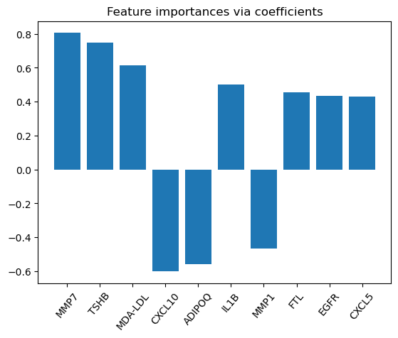
Most important coefficients and features written as a sum

i, j = tup[0]
s = str(round(i, 3)) + " " +str(j)
for i, j in tup[1:]:
    if i < 0:
        sgn = ' '
    else:
        sgn = ' + '
    s = s + sgn + str(round(i, 3)) + " " +str(j)
print(s)

0.805 MMP7 + 0.75 TSHB + 0.614 MDA-LDL -0.602 CXCL10 -0.558 ADIPOQ + 0.502 IL1B -0.469 MMP1 + 0.456 FTL + 0.434 EGFR + 0.431 CXCL5

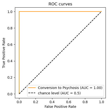
The ROC AUC score

y_score = lr.predict(X)
# Using all the data should result in an AUC near 1
roc_auc_score(Y, y_score)

1.0

ROC curve with an AUC = 1

RocCurveDisplay.from_predictions(
    Y,
    y_score,
    name="Conversion to Psychosis",
    color="darkorange",
)
plt.plot([0, 1], [0, 1], "k--", label="chance level (AUC = 0.5)")
plt.axis("square")
plt.xlabel("False Positive Rate")
plt.ylabel("True Positive Rate")
plt.title("ROC curves")
plt.legend()
plt.show()

The classifier does not learn from the training data.

X_train, X_test, y_train, y_test = train_test_split(
    X.copy(), Y.copy(),
    random_state=42
)

y_score =  LogisticRegression().fit(X_train, y_train).predict(X_test)
# Using all the data should result in an AUC near 1
roc_auc_score(y_test, y_score)

0.48701298701298695