Feature importances with a forest of trees

This example shows the use of a forest of trees to evaluate the importance of features on the N2 classification task. The blue bars are the feature importances of the forest, along with their inter-trees variability represented by the error bars.

Unexpectedly, the plot suggests that no features are informative.

Data and model fitting

input_file = "../../data/n2.csv"

import matplotlib.pyplot as plt
from sklearn.ensemble import RandomForestClassifier
from sklearn.model_selection import train_test_split
import time
import numpy as np
import pandas as pd

df = pd.read_csv(input_file, header=0, sep=",")

# The input data is everything except the first column
X = df.loc[:, df.columns != 'ctrl/case']
# The outcome or diagnoses are in the first ctrl/case column
y = df['ctrl/case']

# The header row is the feature set
feature_names = list(X.columns)

X_train, X_test, y_train, y_test = train_test_split(X, y, stratify=y, random_state=42)

A random forest classifier will be fitted to compute the feature importances.

forest = RandomForestClassifier(random_state=0)
forest.fit(X_train, y_train)

RandomForestClassifier(random_state=0)

In a Jupyter environment, please rerun this cell to show the HTML representation or trust the notebook.
On GitHub, the HTML representation is unable to render, please try loading this page with nbviewer.org.

Feature importance based on mean decrease in impurity

“Feature importances are provided by the fitted attribute feature_importances_ and they are computed as the mean and standard deviation of accumulation of the impurity decrease within each tree.”

Warning

Impurity-based feature importances can be misleading for high cardinality features (many unique values). See permutation_importance as an alternative below.

n_features = 20

start_time = time.time()
importances = forest.feature_importances_
std = np.std([tree.feature_importances_ for tree in forest.estimators_], axis=0)

elapsed_time = time.time() - start_time

print(f"Elapsed time to compute the importances: {elapsed_time:.3f} seconds")

# get the top 10
importances_top, std_top, feature_names_top = zip(*sorted(zip(importances, std, feature_names), reverse=True)[0:n_features])

Elapsed time to compute the importances: 0.014 seconds

Let’s plot the impurity-based importance.

import pandas as pd

forest_importances = pd.Series(importances_top, index=feature_names_top)

fig, ax = plt.subplots()
forest_importances.plot.bar(yerr=std_top, ax=ax)
ax.set_title("Feature importances using MDI")
ax.set_ylabel("Mean decrease in impurity")
fig.tight_layout()

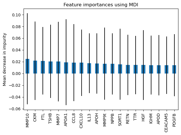
We observe that no features are found important.

Feature importance based on feature permutation

“Permutation feature importance overcomes limitations of the impurity-based feature importance: they do not have a bias toward high-cardinality features and can be computed on a left-out test set.”

from sklearn.inspection import permutation_importance

start_time = time.time()
n_features = 30
result = permutation_importance(
    forest, X_test, y_test, n_repeats=10, random_state=42, n_jobs=2
)
elapsed_time = time.time() - start_time
print(f"Elapsed time to compute the importances: {elapsed_time:.3f} seconds")

forest_importances = pd.Series(result.importances_mean, index=feature_names)

importances_top, std_top, feature_names_top = zip(*sorted(zip(forest_importances, result.importances_std, feature_names), reverse=True)[0:n_features])

Elapsed time to compute the importances: 8.998 seconds

“The computation for full permutation importance is more costly. Features are shuffled n times and the model refitted to estimate the importance of it. Please see permutation_importance for more details. We can now plot the importance ranking.”

fig, ax = plt.subplots()
perm_importances = pd.Series(importances_top, index=feature_names_top)
pd.Series(importances_top, index=feature_names_top).plot.bar(yerr=std_top, ax=ax)
ax.set_title("Feature importances using permutation on full model")
ax.set_ylabel("Mean accuracy decrease")
fig.tight_layout()
plt.show()

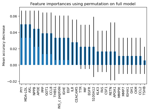
There is little contribution from any of the features.